Gaussian Mixture Models Visually Explained

Introduction

A normal distribution is widely known and used in statistics. Because of the central limit theorem the normal distribution explains the data well in many cases. However, in practice the data distribution might be multimodal, i.e. the probability density function has several ‘bumps’. For example, the distribution of hardcover and paperback books prices, as producing a hardcover book is more expensive.

One way to exploit the nice properties of normal distributions for such multimodal data is to use the Gaussian Mixture Model. This combines several normal distributions with different parameters.

The Gaussian Mixture Model is a generative model that assumes the data is distributed as a Gaussian mixture. It can be used for density estimation and clustering. But, first things first.

Gaussian Mixture

The Gaussian Mixture Model defines a probability distribution on the data of the specific form — the mixture of Gaussians. Though you may rightly ask, “What is the Gaussian mixture exactly?” Gaussian mixture distribution is a linear superposition of m Gaussian components. This is not to be confused with a sum of random variables distributed as Gaussians — this sum is distributed as Gaussian too. Here we sum up not the random variables, but probability density functions with weight coefficients which summing up to 1.

\[\begin{align*} &p(x) = \sum_{k=1}^K \pi_k\; \mathcal{N}\left(\boldsymbol{x} \mid \boldsymbol{\mu}_k, \boldsymbol{\Sigma}_k\right) \\ &0 \leq \pi_k \leq 1 \text { for all } k=1, \ldots, K \\ &\sum_{k=1}^K \pi_k=1 \end{align*}\]

This way we obtain the distribution which comprises of multiple Gaussian components. If the means are far enough, then we might get a distribution with several ‘bumps’, in other words, multimodal distribution. The parameters of this distribution are the weights pi, means, and covariance matrices for each component. The weight coefficients, also called mixing parameters, show how much of the respective component is in the resulting distribution.

To get a better intuition of this, let’s consider the simplest example; when one coefficient is one and all others are zero. In this case, the resulting distribution would be just Gaussian with respective mean and covariance. In a non-degenerative case, the resulting distribution captures all components to some extent. In the figure below, you can see how the resulting distribution changes depending on the value of the mixture parameter.

How to Sample?

We defined this distribution as a combination of multiple Gaussian probability density functions. Equivalently, we can define it as a result of the following sampling procedure.

We first choose a component, and then sample a random variable from the chosen component. In more detail this might look like this:

1. Draw a sample from \( \text{Cat}(\pi)\), which means we choose some \( i\) with probability \(p_i\)
2. Draw a sample from \(i\)-th component, which is from \(\mathcal{N}(\mu_i, \Sigma_i)\)

The sampling procedure is shown in the animation below. The right subplot shows iteratively how many samples are chosen from each component. The resulting histogram is close to the barplot of the weights of components. The left subplot shows the samples drawn from the respective component’s Gaussian distribution. The components contain a different number of points. For example, the upper one (in histogram component 1) contains the least points.

Gaussian Mixture Model

Now imagine we know (or at least assume) the data is generated from the Gaussian mixture. However, the parameters of the distribution remain unknown. How do we learn the parameters? As often in machine learning models, this is done via likelihood maximization (or equivalently, negative log-likelihood minimization).

\[\begin{gathered} \log p(\boldsymbol{X} \mid \boldsymbol{\pi}, \boldsymbol{\mu}, \boldsymbol{\Sigma})=\sum_{i=1}^N \log \left(\sum_{k=1}^K \pi_k\; \mathcal{N}\left(\boldsymbol{x}_i \mid \boldsymbol{\mu}_k, \boldsymbol{\Sigma}_k\right)\right) \\ \boldsymbol{X}=\left\{\boldsymbol{x}_1, \ldots, \boldsymbol{x}_N\right\} \end{gathered}\]

If we had only one component (that would be just a Gaussian distribution) we could take a log. (a gentle reminder: logarithm of the product is just a sum \(\log(ab) = \log(a) + \log(b)\) for \(a, b > 0\)). When we do this the exponent would disappear. Then we take a derivative, set it to zero, and the problem is solved (of course, we noticed that the log-likelihood is concave; hence, the solution is a maximizer).

\[\begin{gathered} \log p(\boldsymbol{X} \mid \boldsymbol{\pi}, \boldsymbol{\mu}, \boldsymbol{\Sigma})=\sum_{i=1}^N \log \mathcal{N}\left(\boldsymbol{x}_i \mid \boldsymbol{\mu}, \boldsymbol{\Sigma}\right)= \\ \sum_{i=1}^N \log \frac{1}{(2 \pi)^{k / 2}|\boldsymbol{\Sigma}|^{1 / 2}} \exp \left(-\frac{1}{2}\left(\boldsymbol{x}_i-\boldsymbol{\mu}\right)^T \boldsymbol{\Sigma}^{-1}\left(\boldsymbol{x}_i-\boldsymbol{\mu}\right)\right)=\ldots \end{gathered}\]

However, in more general cases we have more than one component, and we don’t know the mixing coefficients. Although we still can set derivatives to zero, we won’t obtain a nice closed-form solution.

Let’s note, that if we knew which component a point is from (the class labels) we could learn the parameters of each component independently. Just like how things work when performing the density estimation of normally distributed data. On the other hand, if we knew the parameters of all components, we could assign points to their most probable classes. So, these subproblems are relatively easy to solve. This could lead us to the idea of updating parameters or class labels iteratively based on the previous estimate of class labels or components parameters, respectively. The idea of the EM algorithm is similar, but instead of class labels, it uses responsibilities — probabilities of a point belonging to a cluster.

EM Algorithm

Before we deep dive into the EM algorithm details, I’d like to remind you that this is only one of the approaches to find a maximizer. It can be shown that the algorithm converges, although not always to the global maximum. Another alternative would be, for example, gradient-based approaches.

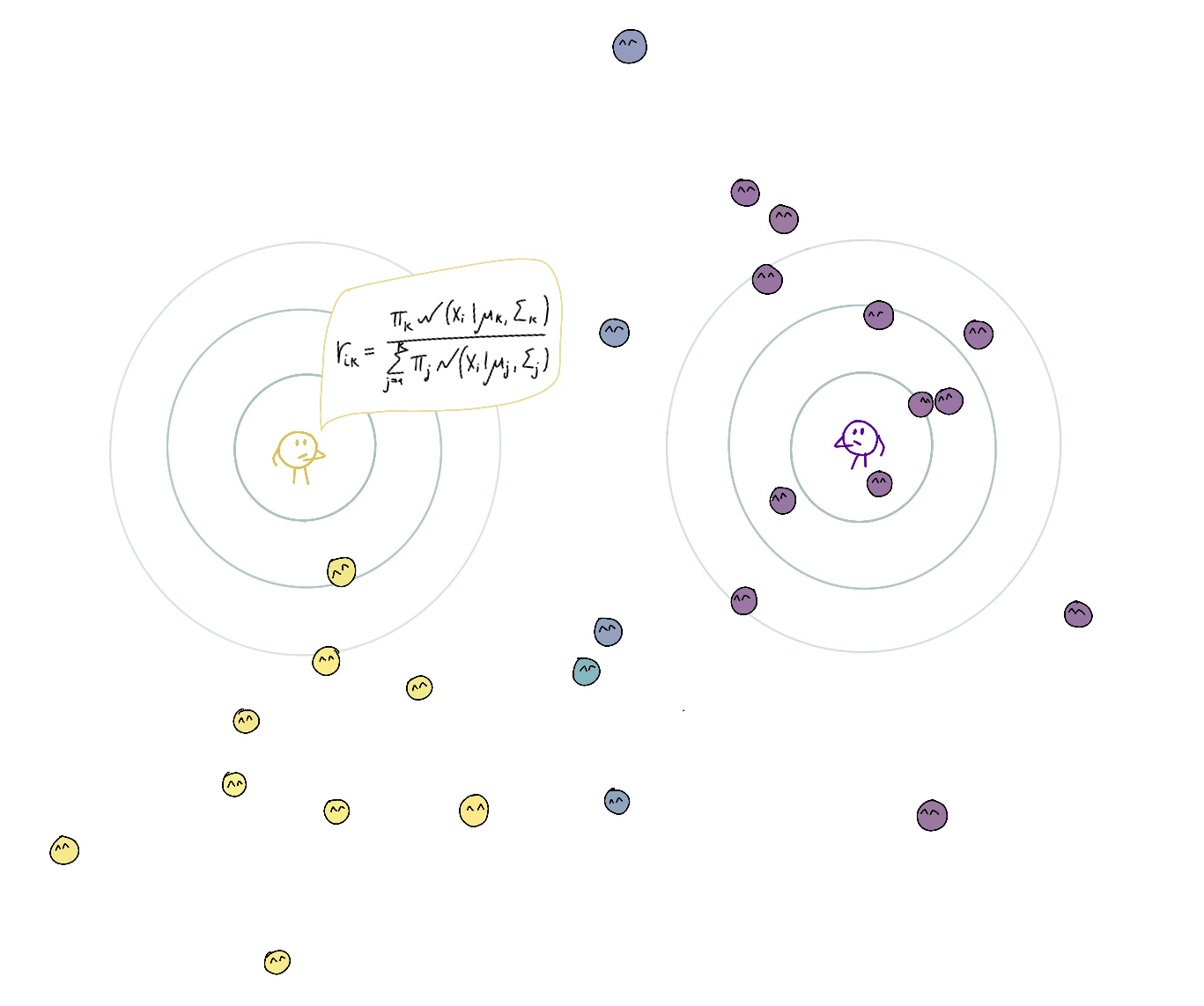
To get further intuition on this, let’s consider an example. Imagine that centers of K clusters are kindergarten teachers looking after points under their responsibility. The teacher’s responsibility for a point depends on the point location, their location (mu), the area they frequently check (zone of responsibility, Sigma), their commitment (pi), and the same parameters of other teachers. The responsibility may be shared between teachers (for example, if a point is between two centers), but the responsibilities for a point of all teachers should sum up to 1. In other words, every point needs to be fully taken care of.

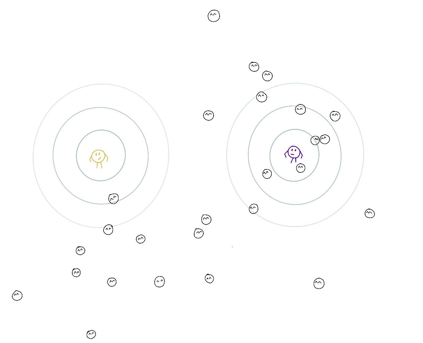
The contours around the teachers are level lines indicating how well they look after points on that line. The further the contour, the more difficult is to check on that location.

The goal is to find locations, zones of responsibility, and teachers’ commitment to increase overall ‘childcare quality’, which is an informal interpretation of likelihood. Another goal is to assign every point to a teacher, whose responsibility for it is largest among other teachers to find groups of points.

The teachers can easily compute their responsibility for all points using the current parameters of all teachers (expectation step).

Then they change the location and their zone of responsibility to better look after the points under their responsibility, moving closer to the points they are mainly responsible for and accounting with lower weight for points they have shared responsibility for (maximization step). Also, their commitment grows with the overall current responsibility.

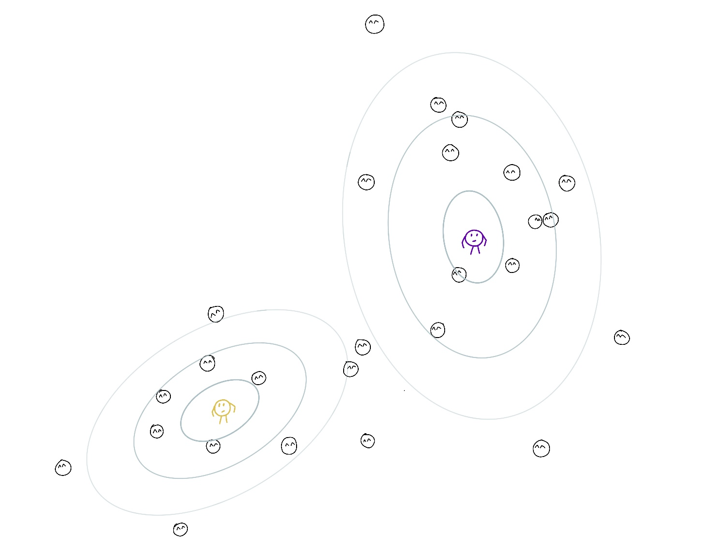
Important point: Even if their responsibility for a point is the lowest among all other teachers (for example 0.2 and 0.8 for another teacher) they still account for it. The objective that they maximize is a weighted version of the log-likelihood with responsibilities acting as weights. The lower the responsibility, the less the respective summand. Hence the lower effect on the parameters of the cluster with low responsibility.

After changing the parameters, they recalculate their responsibilities and move again. The process is repeated until convergence (the changes are so small that the teachers are too lazy to move). It can be shown that the overall ‘childcare quality’ is increasing after each expectation-maximization iteration.

Now let’s move to the formal description of the EM algorithm.

Expectation Step

On the expectation step, we compute responsibilities. The responsibility r_{ik} is the posterior probability that point i belongs to cluster k. It is calculated using the Bayes’ theorem.

\[\begin{gathered} r_{i k}=p\left(z_i=k \mid \boldsymbol{x}_i, \boldsymbol{\pi}_k, \boldsymbol{\mu}_k, \boldsymbol{\Sigma}_k\right)= \\ \frac{\pi_k\; \mathcal{N}\left(\boldsymbol{x}_i \mid \boldsymbol{\mu}_k, \boldsymbol{\Sigma}_k\right)}{\sum_{j=1}^K \pi_j\; \mathcal{N}\left(\boldsymbol{x}_i \mid \boldsymbol{\mu}_j, \boldsymbol{\Sigma}_j\right)} \end{gathered}\]

Maximization Step

As mentioned before, the log-likelihood cannot be maximized in closed form. However, the problem becomes easy once we have class labels. So let’s introduce latent variables Z, i = 1…n, with Z_i being a class label of point i. If we observed both X and Z we could easily deduce parameters of every Gaussian component by maximizing the log-likelihood. However, in our case Z depends on the parameters. Another consideration is that GMM is a probabilistic model, and even if a point is close to the center of a cluster, it could still arise from another cluster with lower probability. When we make inference, we choose the most probable class of each point, but even under GMM assumptions, it doesn’t mean we chose the ‘true’ class.

So now we have the log-likelihood function we want to maximize but cannot compute because of unknown Z… Don’t worry; there’s a solution. One way to estimate a quantity containing randomness is to take its expectation. Although we don’t know Z, we have estimates of its distribution – that’s r_ik computed on the expectation step. We can take expectation of log-likelihood with respect to the posterior distribution of cluster assignments.

\[\begin{gathered} \mathbb{E} p(\boldsymbol{X}, \boldsymbol{Z} \mid \boldsymbol{\pi}, \boldsymbol{\mu}, \boldsymbol{\Sigma})= \\ \sum_{i=1}^N \mathbb{E} \log \left[\prod_{k=1}^K\left(\pi_k\; \mathcal{N}\left(\boldsymbol{x}_i \mid \boldsymbol{\mu}_k, \boldsymbol{\Sigma}_k\right)\right)^{\mathbb{I}\left(z_i=k\right)}\right]= \\ \sum_{i=1}^N \sum_{k=1}^K p\left(z_i=k \mid \boldsymbol{x}_i, \boldsymbol{\pi}_k, \boldsymbol{\mu}_k, \boldsymbol{\Sigma}_k\right) \log \left[\pi_k\; \mathcal{N}\left(\boldsymbol{x}_i \mid \boldsymbol{\mu}_k, \boldsymbol{\Sigma}_k\right)\right]= \\ \sum_{i=1}^N \sum_{k=1}^K r_{i k} \log \left[\pi_k\; \mathcal{N}\left(\boldsymbol{x}_i \mid \boldsymbol{\mu}_k, \boldsymbol{\Sigma}_k\right)\right] \end{gathered}\]

In the second line, we used that only one indicator z_i = k is one, and all others are zero. Therefore, the product contains only one multiplier referring to the true class. The reason to use a product is that we can take it out of the logarithm and obtain a sum.

The maximizers now can be found by setting derivatives to zero and have the following form:

\[\begin{gathered} \pi_k=\frac{1}{N} \sum_{i=1}^N r_{i k}=\frac{N_k}{N}, \text { with } N_k:=\sum_{i=1}^N r_{i k} \\ \mu_k=\frac{1}{N_k} \sum_{i=1}^N r_{i k} \boldsymbol{x}_i \\ \Sigma_k=\frac{1}{N_k} \sum_{i=1}^N r_{i k}\left(\boldsymbol{x}_i-\boldsymbol{\mu}_k\right)\left(\boldsymbol{x}_i-\boldsymbol{\mu}_k\right)^T \end{gathered}\]

The EM algorithm monotonically increases log-likelihood and converges to local maximum. However, this algorithm depends on initialization and is not guaranteed to find the global likelihood maximizer.

Practice

It is a good exercise to implement the EM algorithm for GMM from scratch to check and deepen your understanding. But here, I want to give a quick overview of sklearn implementation usage.

You can find the full notebook at my gmm_visualisation repository.

First, importing libraries and setting matplotlib parameters up:

from sklearn.mixture import GaussianMixture
from sklearn.datasets import make_blobs
import matplotlib.pyplot as plt
import matplotlib
%matplotlib inline
random_seed = 13
scatter_params = {'s': 15, 'alpha': .7}
matplotlib.rcParams['figure.figsize'] = (5, 5)

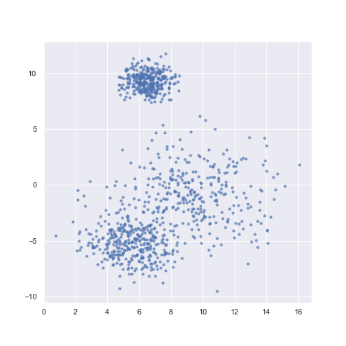
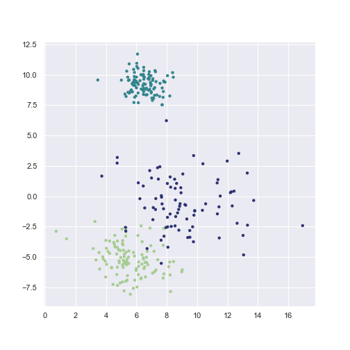
I used simulated data for simplicity and visual clarity.

n_samples = 1000
X, y = make_blobs(n_samples=n_samples, centers=3,
		  cluster_std=[1.5, 0.8, 2.5],
		  random_state=random_seed)
plt.scatter(X[:, 0], X[:, 1], c=y, **scatter_params)

The GaussianMixture() function creates an object, which we then fit to the data to learn the parameters.

gmm = GaussianMixture(n_components=3)
gmm.fit(X)

As was mentioned before, the EM algorithm depends on initialization. In sklearn implementation, results of K-means clustering are used by default for initialization. Another option is setting init_params=‘random’. In this case, responsibilities are initialized randomly using uniform distribution. However, this might lead to non-stable results.

Furthermore, sklearn implementation also allows for regularization, e.g., using the same covariance matrices for all components. It can be done by setting covariance_type=‘tied’ in the initialization of GMM.

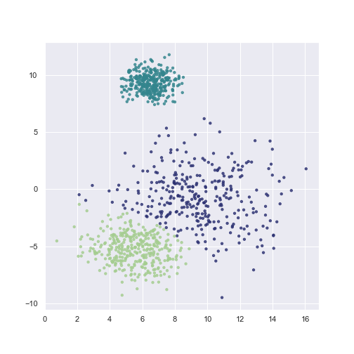
Once we have trained the model, we are ready to make an inference. The fitted GMM object has two options for this task: predict and predict_proba. The first one returns a list of most probable classes of a passed list of points, and the latter returns probabilities of points belonging to a class.

plt.scatter(X[:, 0], X[:, 1], c=gmm.predict(X),
	    **scatter_params)

GMM is a generative model, which means that it can generate new data.

X_sample, y_sample = gmm.sample(300)
plt.scatter(X_sample[:, 0], X_sample[:, 1],
	    c=y_sample, **scatter_params)

Finally, we can use attributes means_, covariances_, weights_ to check the model parameters.

Summary

Why?

• Density estimation
• Clustering

Advantages

• Soft clustering
• Clustering: Captures non-spherical cluster distributions
• Density estimation: Captures multimodal distribution
• EM algorithm for GMM always converges and often works well

Disadvantages

• Requires defining number of clusters
• EM algorithm is dependent on initialization

All animations were made with Python (check my gmm_visualisation repository if you want to see the implementation). The drawings I created in Procreate.